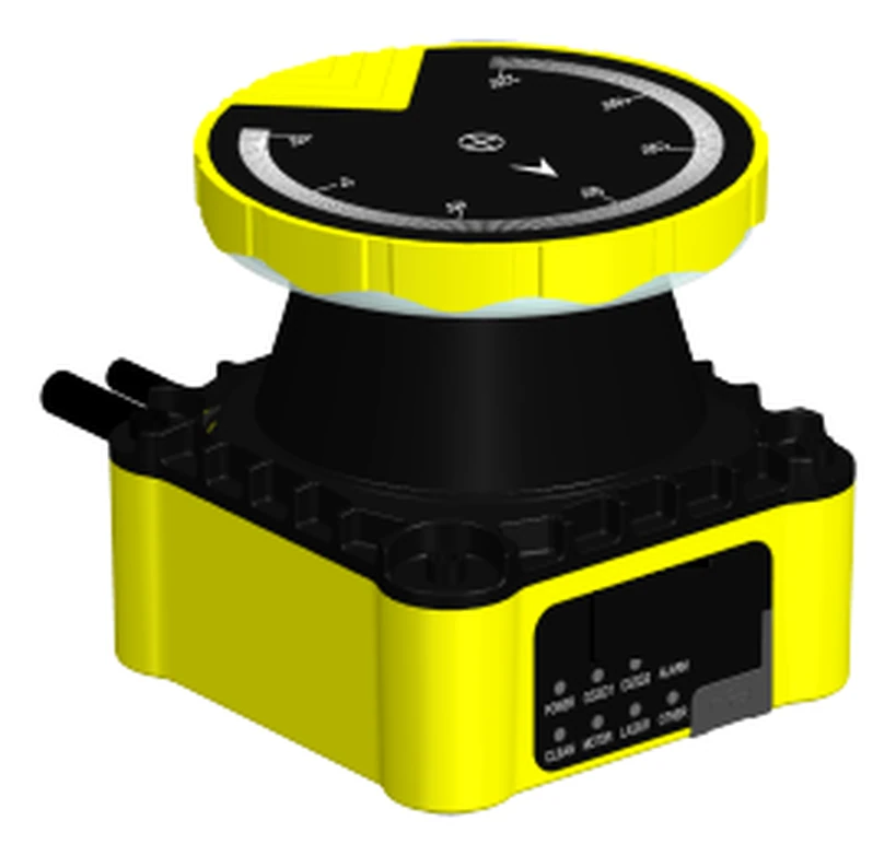
ST27 — Type 3 safety laser scanner, SIL 2 / PL d
5 m protective field · 276° · 100 ms
The only unit here with OSSD outputs and a published rating. Use this one when the scanner has to stop a machine to protect a person.

Use the product groups below to compare models. For a specific engineering question, start with the relevant guide:
Work through the industrial LiDAR selection checklist to compare the task, usable range, outputs and operating limits.
Learn what IEC 61496-3 means for a safety laser scanner before assigning a personnel-protection function.
Follow the factory anti-collision implementation guide to separate ordinary obstacle detection from a validated protective stop.
Review cold-storage AMR scanning and condensation checks when temperature transitions or moisture may affect the application.
The industrial safety LiDAR engineering reference connects terminology, interface checks and application evidence before a specification is sent for quotation.
Start with warning and protective field configuration basics to distinguish operating warnings from a validated safety field and plan commissioning records.
Grouped by the job the scanner does, because the four groups are not interchangeable: a certified safety scanner commands the protective stop, an obstacle-avoidance scanner can trigger ordinary slow-down or alarm logic, and a navigation scanner tells the vehicle where it is. A perception output must not be credited as the personnel-protection safety function.
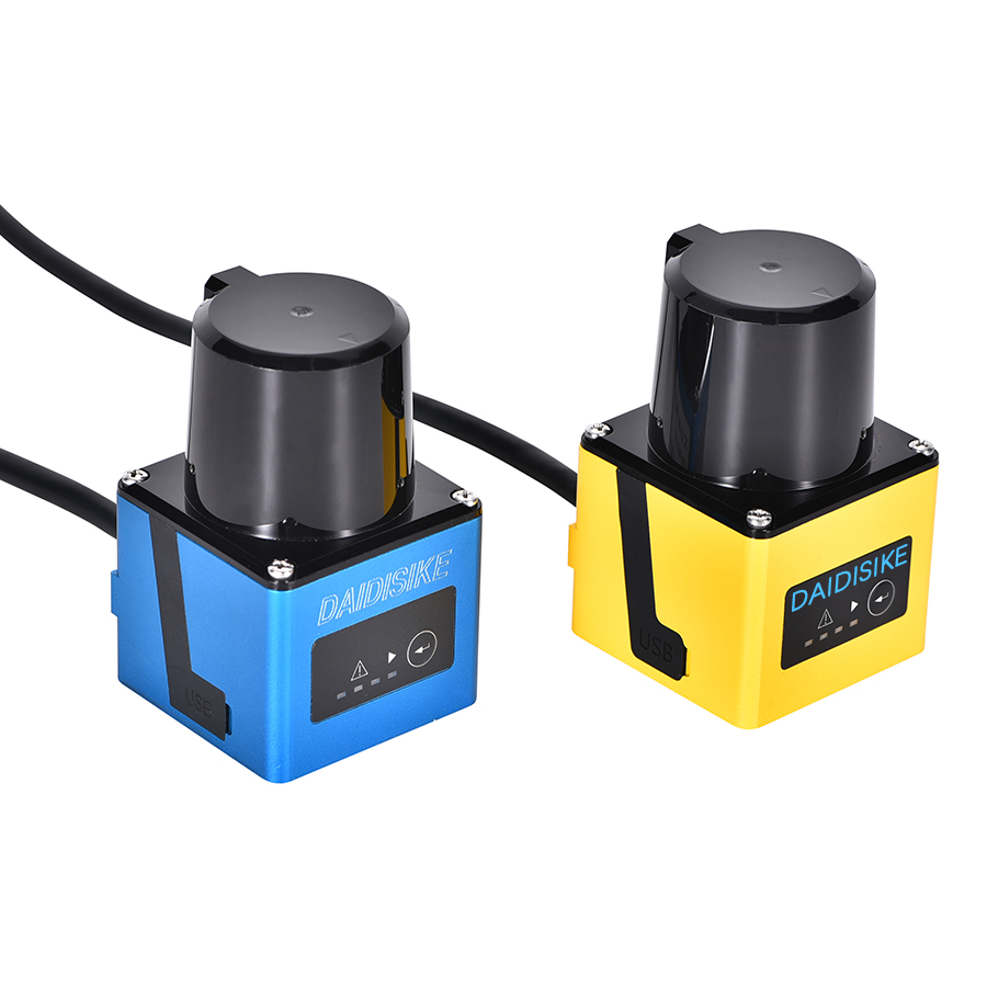
DLD05A3-3N / DLD20A5-5N — 5 m / 20 m obstacle-avoidance LiDAR
0.05–5 m / 0.05–20 m
270° scan, 15/30 Hz. Ordinary AGV/AMR obstacle detection, not the personnel-protection stop.
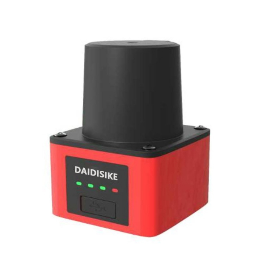
SDLD-05A — 14 m TOF laser radar
up to 14 m
Mid-range avoidance for larger vehicles and wider aisles.
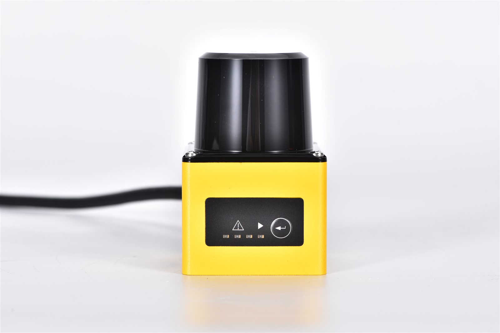
DLDS2030A-5S — 20 m obstacle-avoidance scanning LiDAR
up to 20 m
Zone-based avoidance for machine cells and mobile platforms.
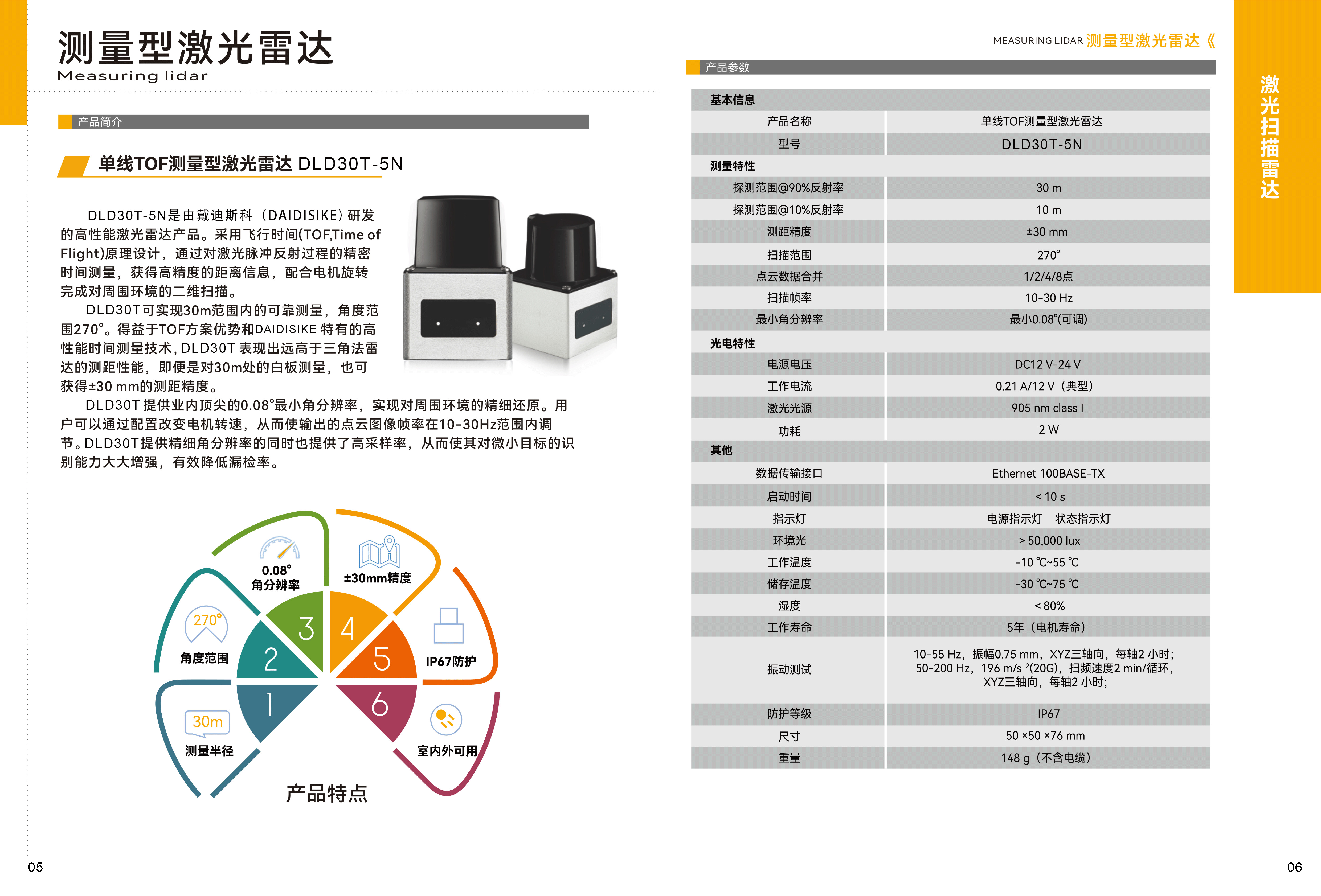
DLD30T-5N — 30 m perimeter-monitoring LiDAR
30 m @ 90% remission / 10 m @ 10% remission
Ordinary perception and perimeter monitoring; Ethernet point-cloud output, not personnel protection.
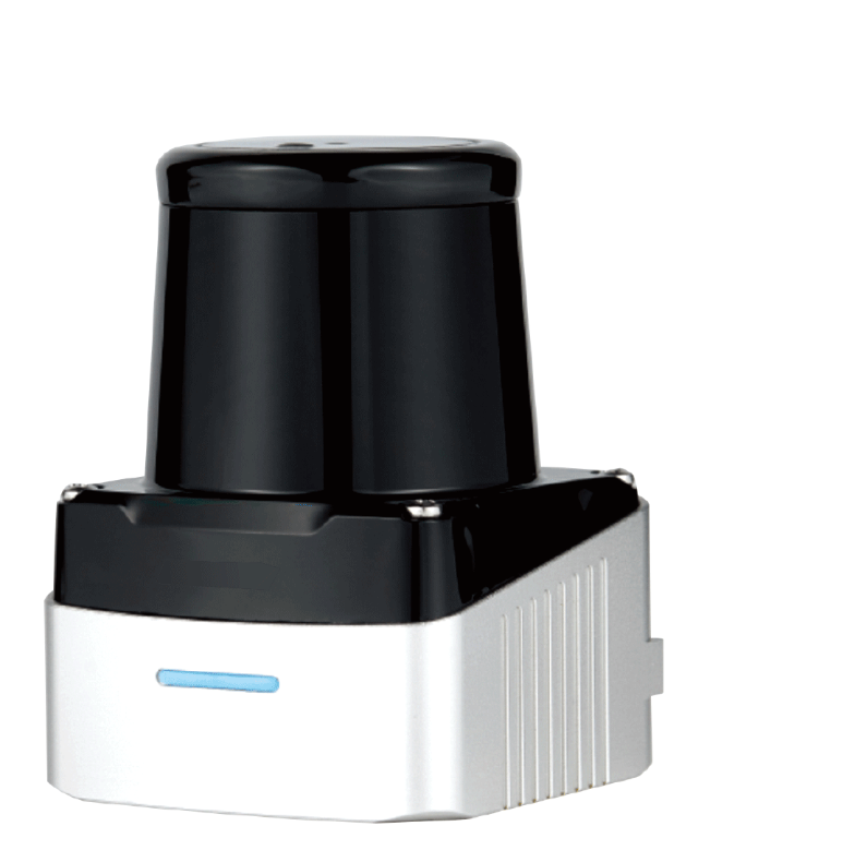
DLD-100D — 100 m TOF scanning laser radar, 280°/360°
up to 100 m
Longest reach in the range; Ethernet output, IP67. Yard and site perimeter.
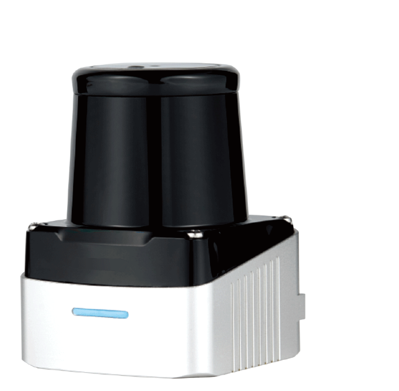
DLD-50D — 50 m 2D TOF LiDAR for SLAM navigation & mapping
up to 50 m
Point-cloud output for a navigation stack — not a stopping device.
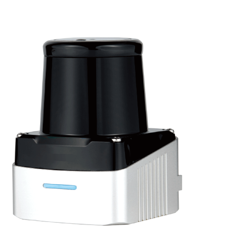
DLD-50G — diffuse-reflective 2D scanning LiDAR, no reflector needed
diffuse, no reflector
Works off the target's own surface, so no retro-reflective tape to install and maintain.
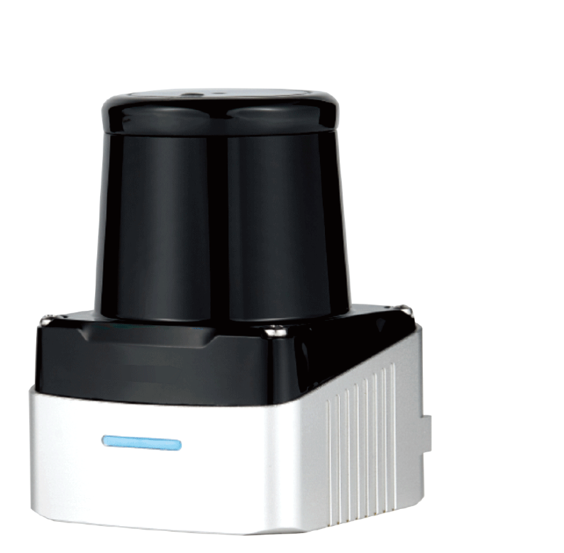
DLD50T8N / DLD50T8P — 50 m measuring LiDAR, NPN/PNP + Ethernet
up to 50 m
Switching output and point-cloud output in one unit — a PLC zone bit without a second sensor.
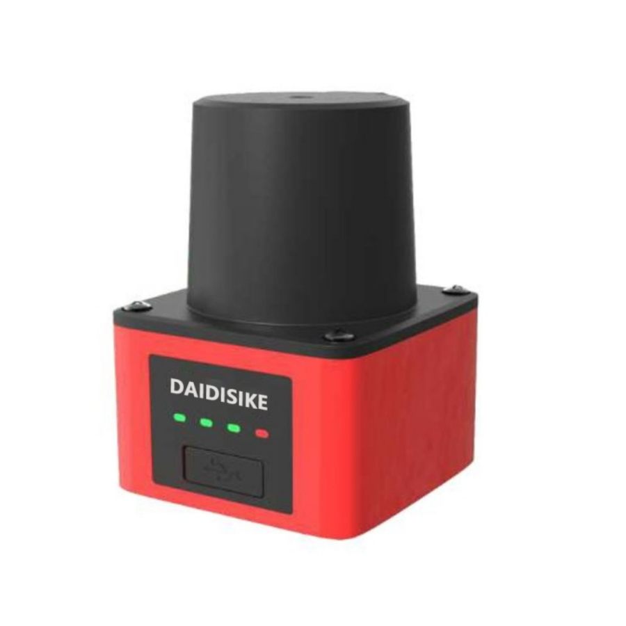
5JPTG / 10JPTG — 5 m and 10 m laser scanning ranging radar
5 m / 10 m
Compact ranging scanners for robotics and light automation.
A LiDAR that draws a zone and switches an output looks exactly like a safety laser scanner. The difference is not visible on the bench, and it can lead to an unsuitable safeguarding design. Two essential checks are:
Where DAIDISIKE stands, plainly: in this range only the ST27 is a certified safety component — Type 3 ESPE per IEC 61496, SIL 2, PL d, with OSSD outputs. Every other scanner on this page (DLD, SDLD, DLDS, JPTG) is a perception and obstacle-avoidance sensor with ordinary switching or Ethernet outputs and no Type, SIL or PL rating. They are the right tool for keeping a vehicle from bumping into things, for area monitoring and for navigation. They are not the right tool for protecting a person, and we would rather say so here than have it discovered during an audit.
The usual architecture on an AMR uses both: a certified scanner for the stop function, and a perception scanner for navigation and for the softer “slow down, something is ahead” behaviour that keeps the vehicle from nuisance-stopping all shift. See the complete AGV/AMR fleet LiDAR integration case for the two-layer architecture and stop-chain boundary.
On a fixed machine, apply ISO 13855 and the scanner manual to the actual approach geometry and stopping time. On an AGV or AMR, field sizing also depends on vehicle motion and measured stopping performance. The following constant-deceleration model illustrates the distance components; it does not replace the applicable vehicle standard or the manufacturer's sizing procedure:
L = v × (tscanner + tcontrol + tbrake) + v² / (2a) + Z
| Term | What it is | Where the figure comes from |
|---|---|---|
| v | Vehicle speed in the direction of travel | Maximum speed permitted for the field set that is active |
| tscanner | Scanner response time | ST27 lists 100 ms; confirm the response time for the selected model and configuration, including any permitted filtering. |
| tcontrol | Safety controller and contactor reaction | From the relay or safety PLC datasheet |
| tbrake | Brake application delay before deceleration starts | Measured on the vehicle, loaded |
| v² / (2a) | Deceleration distance | a = achieved deceleration with the heaviest payload on the worst floor you have, not the empty-vehicle figure |
| Z | Allowances | Scanner measurement tolerance, plus ground-clearance and localisation allowances |
For this illustrative calculation, take a vehicle running at 1.2 m/s, an ST27 at 100 ms, a safety controller adding 30 ms, a brake that takes 150 ms to bite, deceleration of 0.8 m/s² loaded, and 150 mm of assumed combined allowance. The controller, brake and allowance values are example inputs, not ST27 specifications:
Now notice what happens when the fleet manager asks for more throughput. Deceleration distance scales with the square of speed. Using these same example inputs, at 2 m/s the deceleration distance is 2.50 m and the total is 3.21 m. At 2.6 m/s the total is 5.103 m, already beyond a 5 m protective field. These calculations do not establish an approved vehicle speed for the ST27 or any other scanner.
The engineering consequence: if the required field will not fit the operating area or the scanner's rated protective range, review vehicle speed, braking performance, coverage and the safeguarding concept together. Any speed-dependent field selection must be included in the validated safety function.
These are the failures that show up during acceptance testing or, worse, during an incident investigation. They are consistent with what the major scanner manufacturers publish, and none of them are exotic.
The permitted scan-plane height depends on the detection task, object resolution and the exact model's installation instructions. ST27 lists 70 mm object resolution at its maximum protective-field radius. Do not assume that a lower mounting position permits the same safeguarding geometry. Check coverage, access beneath or above the plane and the prescribed test object before accepting the installation.
Multiple sampling sets how many consecutive scans must see an object before the output trips, where that setting is available. Use the exact model's documented settings and response time; there is no assumed default for every scanner. If an approved filtering change increases response time, recalculate the protective field and repeat the prescribed validation tests.
Switching between field sets — slow field in the aisle, long field in the open — affects the safety function. Validate the field-selection inputs and speed monitoring against the required safety performance and the scanner's instructions. A standard PLC signal alone does not establish safe field selection, and a component's rating cannot establish the rating of the complete circuit. Check the response to an incorrect field request.
Compare rated protective range, object resolution, configured response time and environmental limits together. A larger nominal range does not by itself establish better detection in the actual application. Select a model that covers the validated field and test it under the expected operating conditions.
A scanner sees a plane. Corners, forks, overhanging loads and the vehicle's own bodywork cast shadows in that plane. Additional scanners or a different placement may be needed to cover the accessible routes. Verify overlapping coverage and stopping behaviour before finalising the chassis layout.
Dust, steam, rain, snow and fog can affect optical detection and cause faults or nuisance stops. Use the scanner only within its documented environmental limits and check the prescribed response to contamination. Any enclosure or optical cover must be approved for the model; if the conditions fall outside its limits, review the safeguarding technology before commissioning.
Turning “seeing the world” into an engineering capability, LiDAR has traveled more than half a century — from research prototypes to must-have sensors for industrial automation, AGV/AMR navigation, robotic obstacle avoidance, perimeter security, and zone protection. This timeline explains how the technology got here — and answers a practical question buyers and operators care about most: can it stay stable on the line?
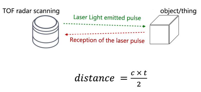
Time of Flight (TOF) made optical ranging practical: emit a laser pulse, measure the round-trip time Δt, and estimate distance as c·Δt/2. Early instruments were bulky and power-hungry, mostly for defense and science. Critical building blocks — semiconductor lasers, photodetectors (APD/SiPM), and pulse shaping — took shape. To turn point measurements into scans, engineers developed repeatable optical mechanisms: spinning mirrors, galvos, and polygon scanners.
Safety baseline: products follow IEC 60825-1 for laser eye safety; most industrial LiDARs target Class 1.
Keywords: laser ranging, TOF, pulsed laser, rotating mirror scanning, photodetection, IEC 60825-1
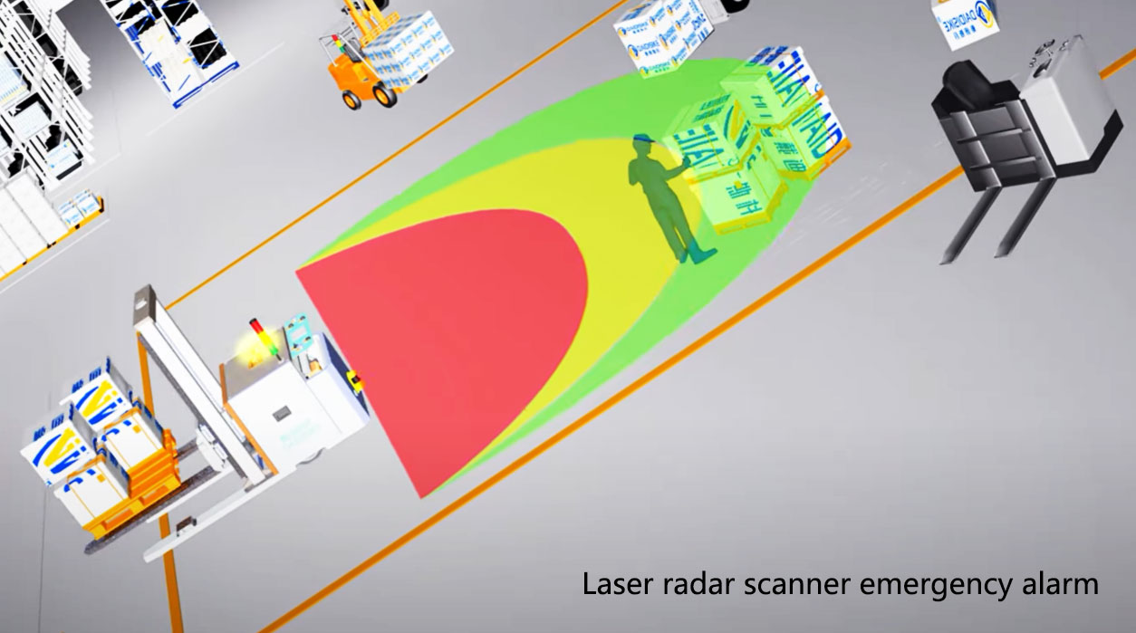
A classic 2D LiDAR pairs a transmitter/receiver with a rotary or oscillating mechanism to build a polar point cloud. Early deployments focused on obstacle detection and zone monitoring: define detection areas and send ordinary I/O to alarm or process-control logic. Personnel protection instead requires a safety-rated scanner and a validated safety interface, controller and stopping chain; ordinary I/O is not that chain.
Functional safety context: LiDARs used in protective functions are commonly engineered with the thinking of ISO 13849-1 (PL), IEC 61508 (SIL), and EN 62061 — risk assessment, redundancy, diagnostics, and verifiable interlocks.
Keywords: 2D LiDAR, scanning rangefinding, zone protection, perimeter security, RS485/Modbus, functional safety
Narrow aisles, glass shelving, and harsh lighting can cause drift or loss when you only have 2D + odometry. The response was multi-beam / solid-state 3D LiDAR plus SLAM (front-end features, loop closure, back-end optimization). The ecosystem matured: ROS/SDK support, multi-sensor fusion (camera + LiDAR + IMU), and native PLC/IPC communications.
Mobile robot safety: ISO 3691-4 raised expectations for obstacle avoidance, speed limits, and emergency stops on AGV/AMR platforms.
Keywords: 3D LiDAR, point cloud, SLAM, AGV/AMR navigation, ROS, ISO 3691-4
The real bar is not hitting spec once, but doing it every shift:
Engineering answers buyers value:
Keywords: glare immunity, low latency, high refresh rate, flexible zoning, IP rating, reliability, fast integration
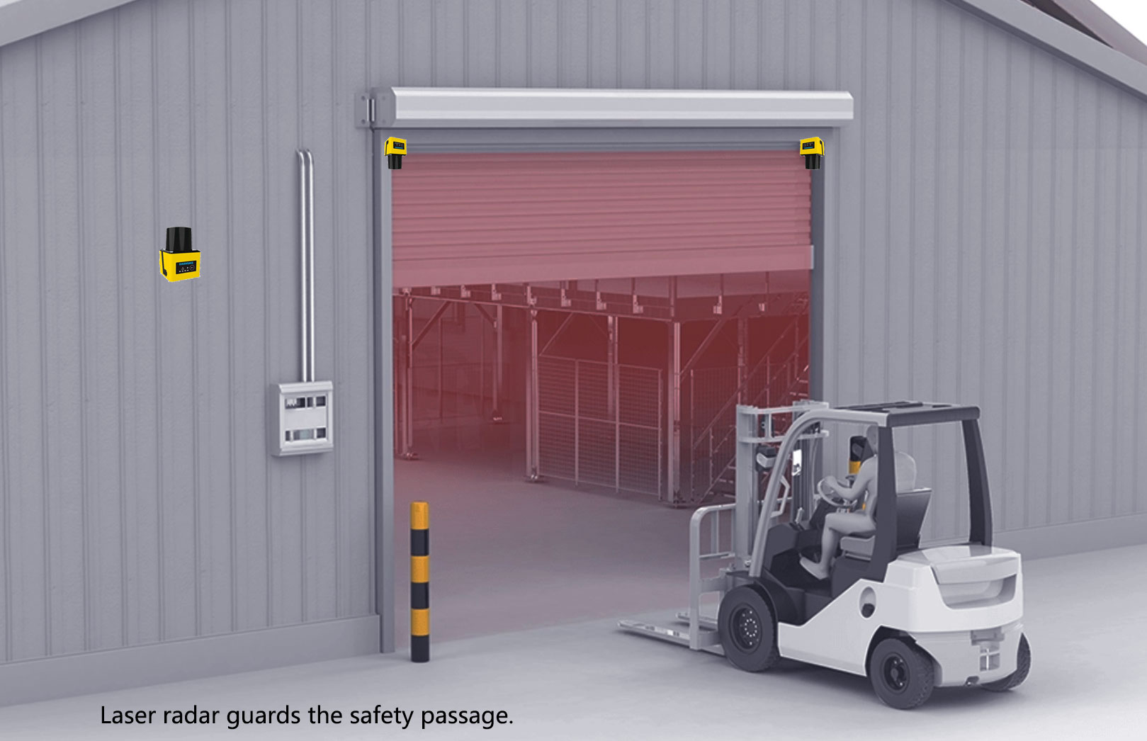
Keywords: industrial automation, AGV/AMR navigation, dynamic obstacle avoidance, perimeter security, EHS, zone protection, false-alarm rate
| Focus | Pragmatic Check | Why It Matters |
|---|---|---|
| Range | Match 5 / 10 / 20 / 30 m… to the actual detection task and target conditions; assess safety protective range separately | Rated range ≠ effective detect distance; reflectivity matters |
| Resolution & Repeatability | Millimeter-class? Edge / thin-object performance | Datasheet specs need robust echo processing to hold up on site |
| Refresh & End-to-End Latency | ≥ 20–30 Hz for fast motion; minimize total latency | Defines the “see → brake” reaction window |
| Interference Immunity | Glare, black surfaces, glass, reflective metals, dust / oil mist | Direct impact on false / missed alarms and maintenance load |
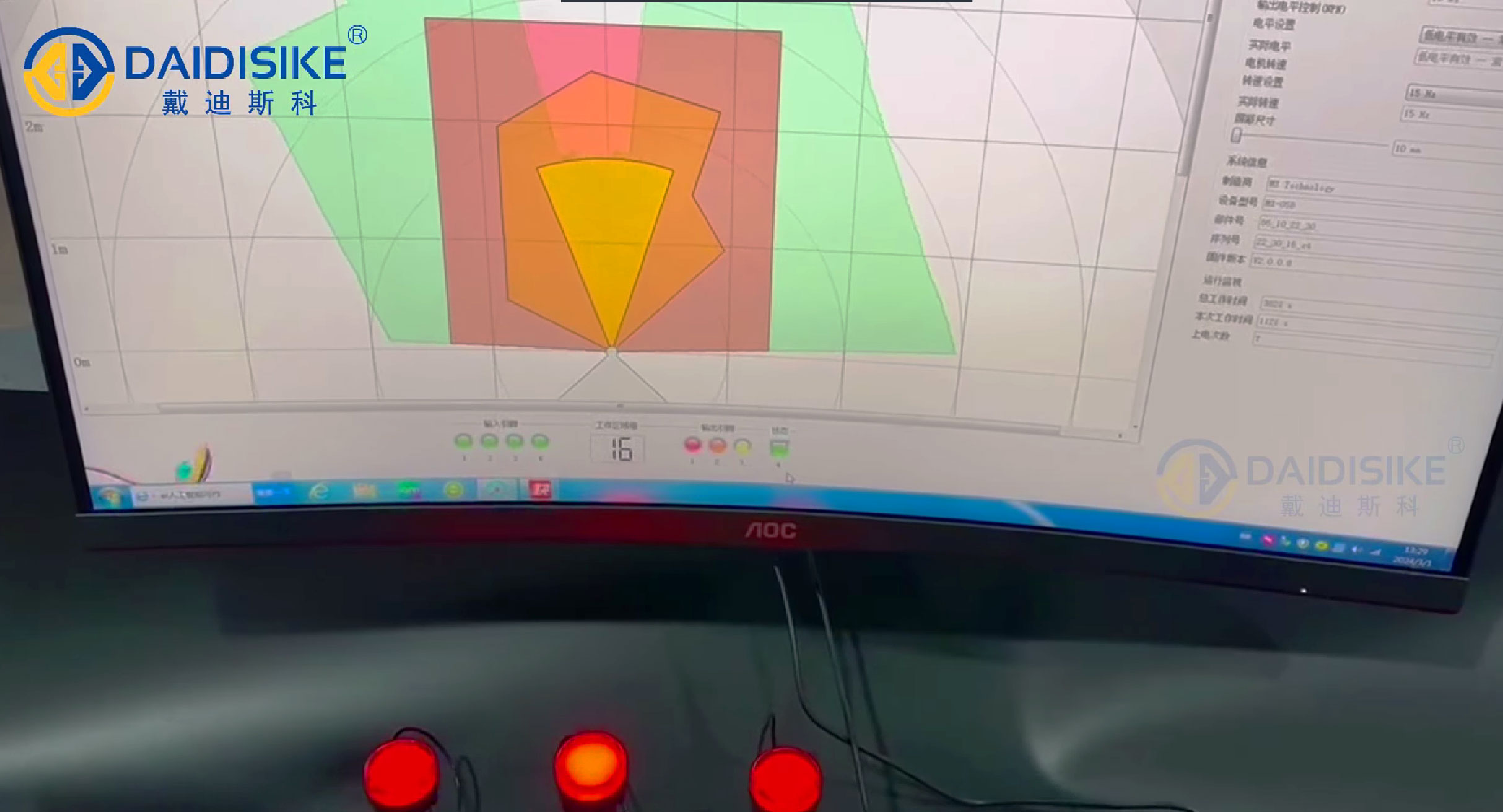
| Zoning Strategy | Separate safety protective fields from ordinary monitoring zones; check supported configuration and logging | Prevents assigning a safety function to non-safety detection data |
| Interfaces & Ecosystem | RS485/Modbus, digital I/O, Ethernet, ROS/SDK | Cuts gateway / dev costs; shortens commissioning |
| Environment Fit | IP rating, vibration, wide temp (e.g. −10–+50 °C), anti-soil | Determines real 24/7 uptime |
| Compliance & Safety | Verify the laser classification separately from Type / PL / SIL and the approved safety interface | Laser emission safety does not establish a personnel-protection function |
Keywords: OEE, data traceability, maintainability, interlock loop, reduced downtime
The story of LiDAR is the story of turning a beam of light into stable capabilities for safety, throughput, and data. Expect continued gains in echo logic, frame rates at lower power, and deeper fusion with vision and ultrasonics. For smart manufacturing and mobile robots, LiDAR will remain a primary viewpoint sensor.
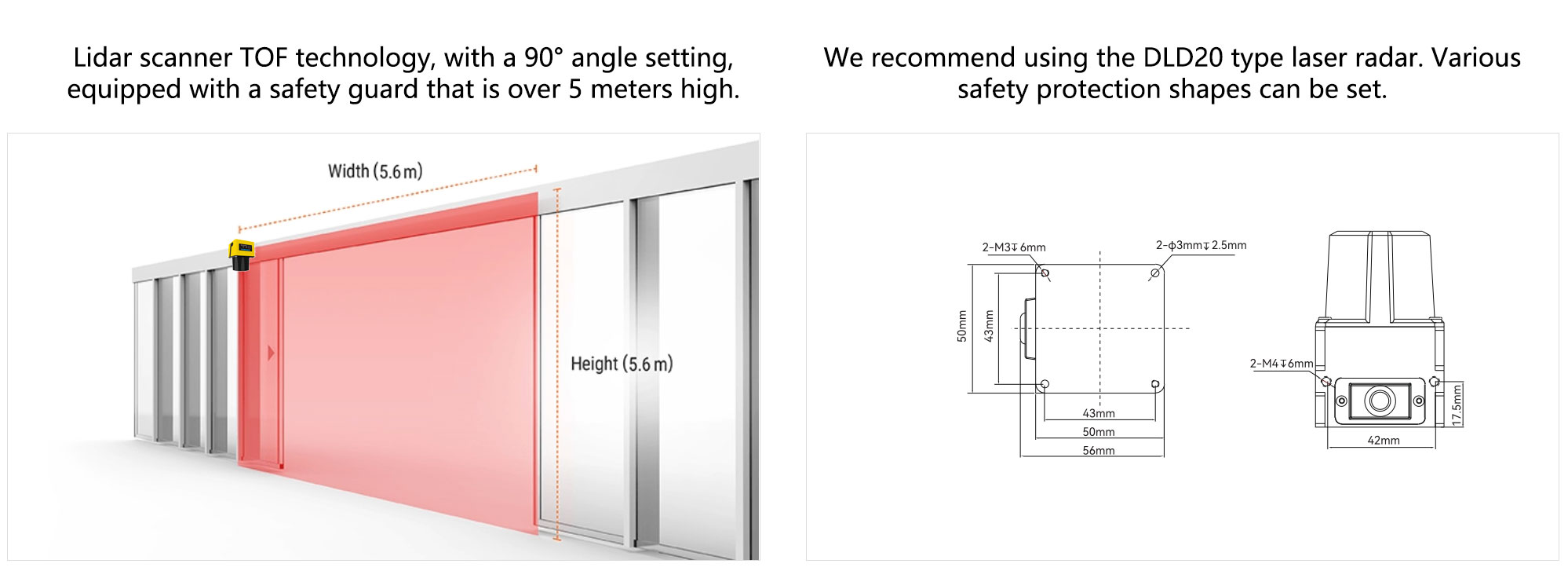
For obstacle detection, zone monitoring, perimeter security, and AGV/AMR navigation, we provide multiple ranges, standard interfaces, and quick-integration options:
DLD05A3-3N / DLD20A5-5N (5 m / 20 m) — Obstacle-Avoidance LiDAR
Use cases: narrow-aisle AGV obstacle avoidance, station presence detection and ordinary machine-area monitoring.
Highlights: configurable detection zones and NPN/PNP switching outputs for warning, alarm or non-safety slow-down logic. See the 5 m vs 20 m AGV obstacle-avoidance LiDAR comparison for model selection.
5JPTG / 10JPTG (5 m / 10 m) — Scanning Rangefinder Radar
Use cases: small mobile platforms, service robots, light-duty AMR.
Highlights: millimeter-class resolution, lightweight, integration-friendly power & interfaces, SDK / protocols for rapid development.
DLD30T-5N — 30 m at 90% remission / 10 m at 10% remission
Use cases: campus / yard channels, semi-outdoor patrol and ordinary long-range zone monitoring; not personnel protection.
Highlights: 270° measurement scan and Ethernet point-cloud data. Use the DLD30T-5N factory specifications to check range, target conditions and integration; do not infer safety outputs or absolute glare immunity.
One-line conclusion: only a certified safety laser scanner such as the ST27 provides Type 3, SIL 2, PL d and OSSD evidence for a personnel-protection stop. General-purpose obstacle-avoidance and navigation LiDARs support detection, mapping and localisation, but they do not perform a safety-rated stop function. Their roles, interfaces and compliance paths are not interchangeable.
For the application path, review how certified safety scanners protect AGVs and AMRs and then use the ANSI/RIA R15.08 mobile-robot safety guide when the project is being validated for North America.
For aisle operation, compare the roles of safety scanners and industrial LiDAR for obstacle avoidance and speed monitoring before assigning navigation signals or protective-stop responsibilities.
| Dimension | Certified Safety Laser Scanner | Navigation / Obstacle-Avoidance LiDAR |
|---|---|---|
| Primary purpose | Personnel protection: entering the protective field switches the verified OSSD safety outputs OFF | Build maps, localise, detect objects or provide ordinary warning / slow-down signals to a controller |
| Output format | Dual-channel OSSD and model-specific diagnostic or safety-network interfaces | Ordinary NPN/PNP switching, point cloud, range or intensity over Ethernet / serial; no OSSD unless the exact model is safety-rated |
| Compliance & safety level | Model-specific Type / PL / SIL evidence; ST27 is Type 3, SIL 2 and PL d | No safety-function rating; not used as the personnel-protection stopping device |
| Engineering metrics | Safety response time, fail-safe behavior, diagnostic coverage, zone switching, immunity to reflections / dust / high ambient light | Angular resolution, scan frequency, range, point-cloud consistency, drift & loop-closure robustness |
| System architecture | OSSD signals feed a verified safety controller or safety relay and the validated stopping chain | The standard controller uses sensor data or switching outputs for navigation, alarm or ordinary slow-down logic |
| Typical placement | Low-mounted / peripheral to cover human ingress risk zones | High or corner mount for complete environmental coverage |
| Typical applications | AMR / AGV safeguarding, forklift retrofits, hazardous-area perimeter guarding, machine guarding | SLAM mapping, localization, path planning, narrow-aisle traversal, global obstacle avoidance |
Mount a certified safety laser scanner low at the front; configure protective / warning fields and speed zones; connect its OSSD outputs to the validated stopping chain.
Mount a navigation LiDAR on the top or corners; feed point clouds to SLAM / localization and planning for corridors, turns, and narrow aisles.
Safety layer has the highest priority. The navigation layer handles speed / path only; once a safety trigger occurs, the vehicle must enter a safe state.
Q1: Can one LiDAR handle both navigation and safety?
A: Use a certified safety laser scanner for the personnel-protection stop and a perception LiDAR for mapping, navigation or ordinary obstacle avoidance. The ST27 is DAIDISIKE's Type 3 / SIL 2 / PL d safety scanner; DLD, SDLD, DLDS and JPTG models are not safety-rated and must not replace it in a safety function.
Q2: How to handle black objects or glass that cause missed detections?
A: Check the exact model's documented remission limits, optical conditions and permitted installation. Test representative dark and reflective surfaces. For a safety scanner, do not add optical film or change its mounting angle or filtering outside the manufacturer's instructions; revalidate the protective field after an approved change.
Q3: How to determine protective and warning field sizes?
A: Determine the protective field from measured stopping performance, configured response times, the approach geometry and manufacturer-specified allowances. Set the non-safety warning field for the application's slowdown or alarm task and validate it separately; a fixed percentage margin is not a universal design rule.
Q4: Do we need re-acceptance after changing sensor models?
A: If a safety-scanner model or protective-field logic changes, repeat the prescribed safety-function validation under controlled conditions, including stopping performance and field boundaries, and archive the approved configuration. Changes to a perception LiDAR need their own detection and control checks; these do not replace safety validation.
Content updated: 2026-09-06. Model selection and engineering validation are separate tasks; ordinary perception outputs are not personnel-safety outputs.